Manipulating Percent Methylation

Kathryn Lande

2024-08-13

While PCBS functions on eigenvector scores internally, users may wish to generate plots using less esoteric values, such as the mean percent methylation difference between conditions. Here we provide a brief tutorial for this type of analysis.

library(PCBS)
library(tibble)
library(tidyr)

Generating a chromDict

chromDicts are lists of keyed data.tables that enable very fast computing times. chromDicts of eigenvector score are used internally by many PCBS functions. They can also be explicitly generated by users who wish to speed up iterative function calls. In order to easily manipulate our percent methylation values genome-wide, we can make a percent methylation chromDict object that holds the average percent methylation difference between two treatments for all filtered loci.

chromDictMethylDiff <- chromDictMeth(eigen, IDs = c("trt", "ctl"), filter_thresh = 50)

Mean methylation over regions

Once the chromDictMeth object is generated, methylation at a region or over a set of regions can be computed very quickly. Get the methylation difference across one known DMR:

MethylDiff(chromDictMethylDiff, "chr3", "4920450", "4923267")
## [1] -0.5493768

Or get the methylation difference across a set of regions:

# we need a data.frame of regions to check:
# any dataframe where the first three column are chrom, start, end, respectively.
regions <- data.frame(chr=c("chr3", "chr3", "chr1"),
                      s=c(4920450, 3961576, 301000),
                      e=c(4923267, 3963805, 303900)) 

regions <- MethyDiff_Set(chromDictMethylDiff, regions)
head(regions) # returns the input file with a "mean_methylDiff" column
##    chr       s       e mean_methylDiff
## 1 chr3 4920450 4923267     -0.54937676
## 2 chr3 3961576 3963805      0.21200740
## 3 chr1  301000  303900     -0.02724904

Metagenes - ∆ Methylation

Like the score_metagene() function, PCBS can also generate metagenes on percent methylation using a chromDictMeth object.

methylDiff_metagene(chromDictMethylDiff, regions)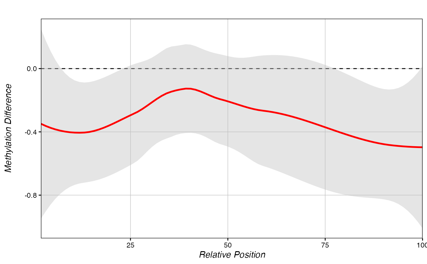

Just like score-based metagenes, you can save the data from a methylDiff_metagene() function and overlay multiple metagenes on a single plot.

# Some hypomethylated sites:
hyper <- data.frame(c=c("chr1", "chr3"),
                    s=c(8650728, 3960576),
                    e=c(8652017, 3962805))

# Some hypermethylated sites:
hypo <- data.frame(c=c("chr3", "chr3", "chr3"),
                   s=c(4920450, 4140014, 1340221),
                   e=c(4923267, 4142951, 1342791))

metagene_hyper <- methylDiff_metagene(chromDictMethylDiff, hyper, return.data = T)
metagene_hypo <- methylDiff_metagene(chromDictMethylDiff, hypo, return.data = T)

multiple_metagenes(data_list = list(metagene_hyper, metagene_hypo), # list of raw data
                   set_names = c("Hyper DMRs", "Hypo DMRs"), # names for elements of the data_list list
                   title="Metagenes of DMR Regions", legend.title = F, 
                   yaxis = "Mean Methylation Difference")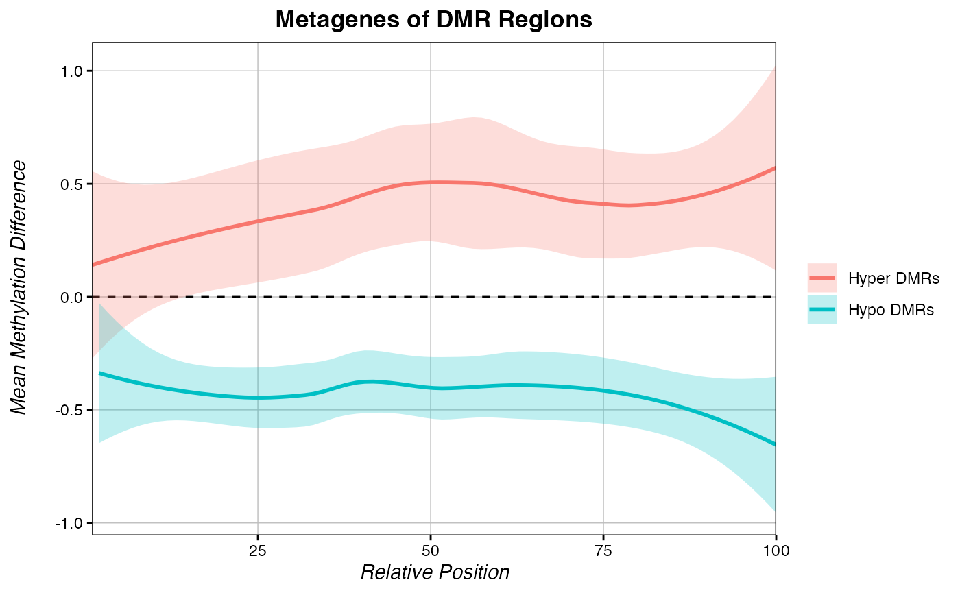

Metagenes - Other Values

More broadly, we can make a chromDict of essentially any value, and by extension, a metagene of essentially any value. The chromDict() function only needs a single column dataframe, where genomic loci are row.names. For example:

# we need a data.frame of regions to check:
head(getPCRanks(eigen, c("trt", "ctl")))
##                   PC_Score
## chr2:2505718  3.781088e-05
## chr2:1807326  4.573342e-04
## chr2:2490208  3.156102e-03
## chr2:5512828 -5.695585e-03
## chr3:1296629  2.822282e-03
## chr3:3212276 -6.044066e-03

Normally, this function takes the PC score, but we can also feed it another value, such as total coverage:

# we need a data.frame of regions to check:
eigen$meanCounts <- rowMeans(eigen[which(grepl("nCpG", colnames(eigen)))]) # the column in our dict will be called "totalCounts"
eigen <- eigen %>% column_to_rownames("cpgID")
head(eigen[c(13)])
##              meanCounts
## chr2:2505718   56.50000
## chr2:1807326   59.83333
## chr2:2490208   57.33333
## chr2:5512828   46.16667
## chr3:1296629   55.83333
## chr3:3212276   53.50000

Then we can make a metagene of coverage:

# we need a data.frame of regions to check:
coverageDict <- chromDict(eigen[c(13)])

# metagenes on alternative values are made the same way, but the added "value" parameter must be specified. 
methylDiff_metagene(coverageDict, hyper, 
                    yaxis = "Total Sequencing Depth", # y-axis name is "Methylation Difference" automatically
                    value = colnames(coverageDict[[1]])[1]) # column name for the plotted value inside your dict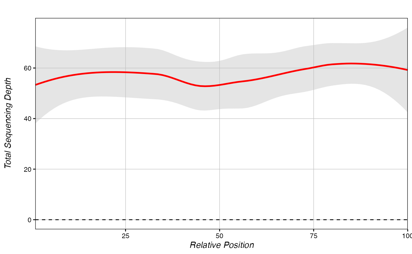

We can also make separate chromDicts for the treatment and control samples. This way, we can plot the mean methylation in young and old separately:

# matrix of percent methylation only:
eigen[which(grepl("PercMeth", colnames(eigen)))] -> eigen_meth

# take the mean of "trt" and "ctl" columns separately:
eigen$trt_mean <- rowMeans(eigen_meth[which(grepl("trt", colnames(eigen_meth)))])
eigen$ctl_mean <- rowMeans(eigen_meth[which(grepl("ctl", colnames(eigen_meth)))])

# make dicts for trt and ctl:
trt_Dict <- chromDict(eigen["trt_mean"])
ctl_Dict <- chromDict(eigen["ctl_mean"])

# make metagenes for each dict separately:
metagene_trt <- methylDiff_metagene(trt_Dict, hyper, return.data = T, value = "trt_mean")
metagene_ctl <- methylDiff_metagene(ctl_Dict, hyper, return.data = T, value = "ctl_mean")

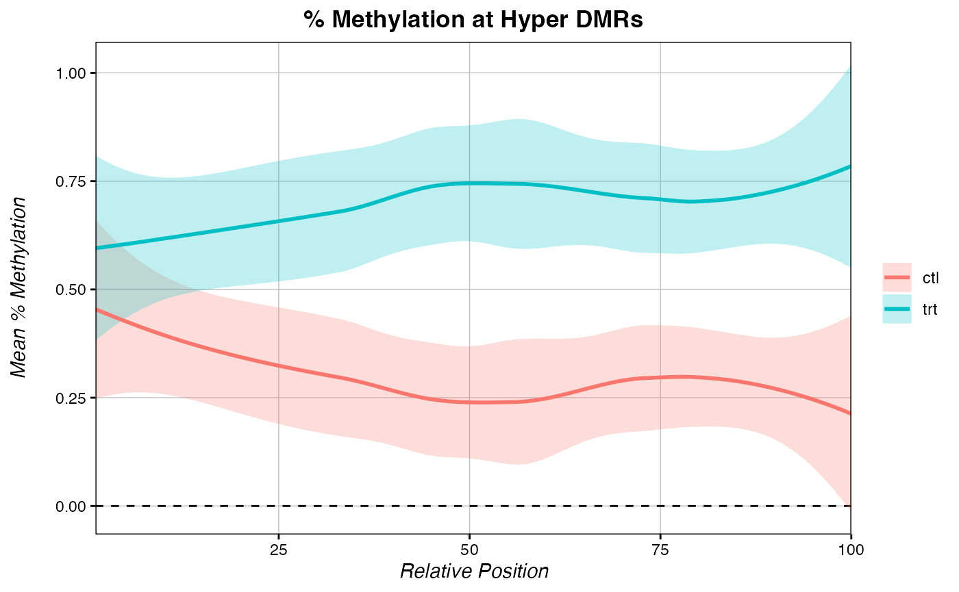
# plot metagenes of % methylation at hypermeth sites in each condition separately:
multiple_metagenes(data_list = list(metagene_trt, metagene_ctl), # list of raw data
                   set_names = c("trt", "ctl"), # names for elements of the data_list list
                   title="% Methylation at Hyper DMRs", legend.title = F, 
                   yaxis = "Mean % Methylation")